How do you measure the accuracy of a classifier?
S. Sochacki, PhD in Computer Science
A2D, ZA Les Minimes, 1 rue de la Trinquette, 17000 La Rochelle, FRANCE
1 INTRODUCTION
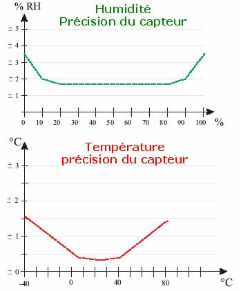
We always consider that a method will never be optimal for all the individuals it treats. In metrology, for example, we know that the accuracy of a sensor is not constant over the band of values it can accept, as illustrated by figure 1.1 showing the evolution of the accuracy of a humidity and temperature sensor used in meteorology. We can see very clearly that measurement accuracy is lower at the extremes.
In order to provide the user with information on the quality of the decision, we need to take into account all possible measures of accuracy, recorded at each stage of processing before arriving at the final decision. When it comes to classification, what can be measured at the output of a classifier? Is it its accuracy? If so, can we use this measure to dynamically select a classifier in order to optimize computation times and recognition performance?
To detail our work, let’s first take a look at what a classifier is and what measurements can be made on a classifier according to the literature (part 2). From there, part 3 presents different ways of dynamically selecting a classifier. We’ll then look at the data we’ve been working with and our various results in part 4. Part 5 will be devoted to the study of these results and part 6 to the conclusion of this article.
2 CLASSIFIERS
The Trésor de la Langue Française defines classification as “the systematic division into classes, categories, of beings, things or notions having common characteristics, particularly in order to facilitate their study”. We therefore define a classifier as an automatic tool, an operator, performing a classification.
From a mathematical point of view, a classifier is an application from an attribute space  (discrete or continuous) to a set of labels
  .
.
Classifiers can be fixed or learning, and these in turn can be divided into supervised or unsupervised learning classifiers.
Applications are numerous. They can be found in medicine (analysis of pharmacological tests, analysis of MRI data), finance (price prediction), mobile telephony (signal decoding, error correction), artificial vision (face recognition, target tracking), speech recognition, datamining (analysis of supermarket purchases) and many other fields.
An example is a classifier that takes a person’s salary, age, marital status, address and bank statements as input, and classifies a person as eligible/not eligible for credit.
A classifier is based on a priori knowledge (fixed by the expert or constructed by learning) describing the different classes in the attribute space. Based on this knowledge, the classifier assigns to the unknown individuals presented to it the label of the class to which the individual has the highest probability of belonging.
It’s important to remember that a single classifier can’t guarantee ideal performance in all possible cases (overlapping class models, individuals at the boundaries between several classes, etc.). This is why it’s a good idea to combine several classifiers so that they can compensate for each other’s errors.
Zouari proposes a taxonomy (see figure 2.1) of different combination methods in [38].
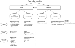
In particular, she reports on the work of Parker[26], which shows that rank-based methods can outperform class-and-measure methods. She also explains that non-parametric methods are the most widely used by researchers, as they are simple to implement and require no additional processing (learning). In addition, they are often the quickest to code and, above all, independent of class structures.
The aim of classification is to establish order relationships between individuals, in order to obtain the most concise information possible, reaching the highest level of abstraction (i.e. to describe, in a precise way, a 3MB document in 100kb). There is a space that describes known data, but how do you choose it?
A classifier can be seen on the one hand as a distance measure, and on the other as a spatial organization method (with an optimization method in the background). Combined, these two parts make the classification operator a tiling operator in the representation space of the data proposed to it. This leads to questions such as, given a distance, what is the best organization?
The role of the classifier is twofold:
- Analyze data without learning (without supervision): create groups, set up an organization;
- Position individuals in relation to groups with learning (with supervision): local information about the individual.
In more general terms, we want to create groups that respond to expectations of use or interpretation, artificially creating them according to common characteristics, with the choice of criteria constraining the choice of space. But how do we choose these criteria?
Automatic classification techniques produce groupings of objects (or individuals) described by a number of
variables or characters (attributes). The use of such techniques is often linked to assumptions, if not requirements
about the groupings of individuals. There are several families of classification algorithms, as described in[22] :
- Partitioning algorithms
- Bottom-up (agglomerative) algorithms
- Top-down (divisive) algorithms
Each of these methods has its own advantages and disadvantages, which are why they are selected according to the application context. Of course, these aspects also justify the combined use of classifiers. A whole community organized around the world of learning has been created to combine several classifiers in a single application. However, in our context, these combinations are defined as static, as they are established a priori to the final decision, at the end of the learning process.
Without repeating the argument that the same operator may have difficulty in being adapted to all the cases posed by the application, we come here to the same conclusion concerning static combinations of classifiers. Of course, this is not an absolute truth, as the quality of the results obtained by these static classifier combination techniques for certain applications is not in question. However, in applications where data variability is very high, static assembly may have difficulty in achieving a high level of results.
In the hypothesis of dynamic combination of classifiers, we know that there are both issues of dynamic selection of the best classifier and, in our thinking, those of estimating a measure of accuracy to be associated with the classification result.
To get us started on these issues, we will draw on the work of L. Kuncheva[20][18][19], who has studied and developed a set of tools for measuring the quality of a classifier in relation to other classifiers, and then presents a measure (diversity) of a classifier’s contribution to a group of classifiers.
2.1 QUALITY MEASUREMENT IN THE LITERATURE
Estimating the quality of a classifier’s results is often based on a posteriori analysis of the propensity of classifiers to make mistakes. When classifiers are compared with each other, quality is estimated on the basis of the rate of correct classification. These comparisons can be based on the same criteria as for a single classifier (good/bad recognitions, etc.), but can also use tools inspired by statistics to measure the quality of a model, a probability law, etc.
In the search for what might constitute an estimate of decision accuracy or of the elements involved in the dynamic combination of classifiers, we have analyzed various criteria associated with decision quality. We propose some of these criteria below:
- The calculation of a classifier’s error, which corresponds to the number of misclassified individuals out of the total number of individuals. Expressed as a probability, it becomes possible to select classifiers according to their probability of making an error within a confidence interval.
- Comparison between 2 classifiers: if 2 classifiers give different error rates on the same test base, are they really different?
- Let’s consider 2 classifiers, and their performances,
 the number of individuals correctly classified by the 2,
  the number of individuals misclassified by the first but well classified by the second,
  the opposite and
  the number of individuals misclassified by the 2. There is a statistical variable following a Chi-square distribution, measuring the quality of one classifier compared to another, written as:
*** QuickLaTeX cannot compile formula:
\begin{equation*}
x^2=\frac{(|N_{01}-N_{10}|-1)^2}{N_{01}-N_{10}}
\end {equation*}
Knowing that $x^2$ is roughly distributed according to $\chi^2$ with 1 degree of freedom, we can say, with a certainty level of 0.05, that if $x^2$>3.841, then the classifiers perform very differently. Note that there is also a test called "difference of two proportions", but Dietterich proves in [4] that this measure is too sensitive to violation of the data independence rule (problem of the restricted learning and recognition dataset) and recommends using the above measure. </li>
</ul>
</li>
 	<li>Several authors have extended this comparative analysis to the case where several classifiers are combined from the same learning base [35] :
<ul>
 	<li><strong>Cochran's Q Test</strong>[8][21] tests the hypothesis: ''all classifiers perform equally well''. If the hypothesis is verified, then
\begin{equation*}\tag{2.1.2}
Q_c=(N_c-1)\frac{N_c\sum_{i=1}^{N_c}G_i^2-T^2}{N_cT-\sum_{j=1}^{N_x}(N_{cj})^2}
\end {equation*}
The variable $Q_c$ follows a $\chi^2$ with $N_c-1$ degrees of freedom, with $G_i$ the number of elements of $\mathcal{L}$ (learning space) correctly classified by the classifier $C_i(i=1,...,N_c)$, $N_x$ being the total number of learned individuals. N_{cj}$ is the total number of classifiers in $\mathcal{C}$ who correctly classified the object $x_j\in \mathcal{L}$ and $T$ is the total number of correct decisions made by all the classifiers.Thus, for a given confidence level, if $Q_c$ is greater than the expected value of $\chi^2$ then there are significant differences between the classifiers justifying their combination. </li>
 	<li>The same principle can be adopted by adopting a Fisher-Snedecor distribution with $(N_c-1)$ and $(N_c-1)*(N_x-1)$ degrees of freedom. This is the <strong>F-Test</strong>[23]. Starting from the performance of the classifiers estimated during training $(\bar  {p_1},...,\bar{p_{N_c>$ and the overall average performance $bar{p}$ we obtain the sum of squares for the classifiers :
\begin{equation*}\tag{2.1.3}
SSA=N_x\sum_{i=1}^{N_c}\bar{p_i}^2-N_xN_c\bar{p}^2
\end{equation*}

*** Error message:
Missing $ inserted.
leading text: ...he total number of learned individuals. N_
File ended while scanning use of \mathaccentV.
Emergency stop.
Then the sum of squares for the objects:
(2.1.4)

The sum total of squares:
(2.1.5)

Finally, the sum total of squares for the classification/object interaction:
(2.1.6)

From then on, the
 criterion is estimated as the ratio between the MSA and the MSAB defined as follows:
(2.1.7)

- It is also possible to apply cross-validation[4]. This involves repeating the learning/recognition process a certain number of times (
 ), each time splitting the dataset to be learned into 2 subgames (usually 2/3 of the data for training and 1/3 for testing). Two classifiers
  and
and  are trained on the training set and tested on the test set. In each round, the accuracies of the two classifiers are measured:
  and
and  . We thus obtain a set of differences, from
  to
to  . Assuming
  , we measure :
(2.1.8)

If
 follows a Student’s distribution with
  degrees of freedom (and for the chosen confidence level), then both classifiers behave in the same way.
- Let’s consider 2 classifiers, and their performances,
Let’s recall that the aim of this work is to achieve a dynamic classification operator selection system, based on a quality measure. The methods presented above have a number of drawbacks when it comes to meeting our needs:
- As far as measuring the error of a classifier is concerned, this information is non-uniform over the attribute space. Moreover, we can assume that this information will vary if we increase the size of the learning space over time.
- Classifier comparison methods require a large number of training and test sessions. Beyond comparisons, once a measure has been established, how do we decide which classifier to use? In the case of cross-validation, if we run 10 trials, we build 10 different classifiers, constructed on 10 different subsets. The sole purpose of these methods is to give an estimate of the accuracy of a certain model built solely on the present problem. Dietterich, in [4], hypothesizes that classification accuracy varies with the size of the training set.
Kuncheva proposes an approach that considers a set of elementary classifiers as a single classifier, built and tested on the same training and test sets.
2.2 DIVERSITY: A SOLUTION?
2.2.1 DEFINITION
We have to admit that each classifier makes errors, otherwise what would be the point of combining them? From there, we seek to compensate for the errors of one classifier by combining it with another, which will produce errors but on different objects. In this way, the diversity of a classifier’s outputs becomes a crucial element for successful combination. Intuitively, we can say that, seeking to obtain the best possible quality output, if there are errors, it’s better that these errors fall on different objects from one classifier to another. Kuncheva explains that, in practice, it’s very difficult to define a single diversity measure, and even more complicated to link this measure to ensemble performance in one simple dependency expression. While there are diversity measures specific to certain branches of science (biology, software design, etc.), we will focus on those that concern classifier ensembles. Diversity can be considered from 3 different points of view:
- As a feature of the set of classifiers: We have a set of classifiers, but we don’t know which combination method to use, and we don’t even know if the decisions given are correct. In this case, diversity provides additional information on individual error rates and overall error. Diversity allows us to discover whether or not a classifier contributes to the success of the ensemble.
- As a characteristic of the set of classifiers and their combination: In this case, we know the set of outputs. So we can tell which classifier deviates the most and which the least from the rest of the ensemble, and measure diversity on a more individual basis. Different combinations will lead to different diversities for the same set of classifiers.
- As a characteristic of the set of classifiers, their combination and the errors: we can finally use the a priori known information of the class to which the individuals in the training set belong (this information is also called the oracle). Diversity is considered as a component of the error set. This is the current focus of Kuncheva’s work[19]: discovering a relationship between diversity and the error set in order to build better combinations.
Before discovering the various measures of diversity, let’s recall the following notations:
- Mathcal{T}
 \mathcal{T}=\{x^*_1,x^*_2,…,x^*_{N_{x^*}}\}
 : decision of classifier
  for individual
  .
.  : Number of classifiers
 : accuracy or probability for classifier to give the right answer
 : space of classifiers
 : number of unknown individuals
2.2.2 DIVERSITY MEASUREMENT USING CLASSIFIER PAIRS
- Disagreement measure: probability that two classifiers disagree on their decisions
- Double fault measure: probability that the classifiers are both wrong
2.2.3 OTHER DIVERSITY MEASURES
- Measure of entropy: considering that the set is more diverse if for a particular individual, half the votes are 0 and half are 1, and similarly that diversity is zero if all classifiers agree, a possible measure of this concept is:
(2.2.3.1)
![\begin{equation*} E=\frac{1}{N_{x^*}}\frac{2}{N_c-1}\sum_{j=1}^{N_{x^*}}\min[(\sum_{i=1}^{N_c}C_{i}(x^*_j)),(N_c-\sum_{i=1}^{N_c}C_{i}(x^*_j))] \end{equation*}](https://www.a2d.ai/wp-content/ql-cache/quicklatex.com-d4e398d723f5638b951f70aea9bc0c2c_l3.png "Rendered by QuickLaTeX.com")
E
 Y(x_j^*)
 x_j^*
x_j^*
KW
 \overline classifiers{D}
KW

X
 {0/N_c, 1/N_c,…, 1}
 \mathcal classifiers{C}
 x^*
x^* N_c
N_c \mathcal{C}
 \mathcal{T}
 X
X X
X Y
Y x^*(x\in \mathcal{T})
 p_i
p_i Y=i/N_c
 i
i N_c
N_c p(i)i
p(i)i x^*
x^* \mathcal{T}
 p(2)=0
 p(1)
p(1) p(1)=\sum_{i=1}^{N_c}\frac {i}{N_c}p_i
 p(2)=\sum_{i=1}^{N_c}\frac{i(i-1)}{N_c(N_c-1)}
GD
![, in order to obtain a minimum value of 0 when all classifiers are always right, or when they all simultaneously give either a right or a wrong answer: <span class="ql-right-eqno"> (2.2.3.7) </span><span class="ql-left-eqno"> </span><img src="https://www.a2d.ai/wp-content/ql-cache/quicklatex.com-db118424e4065f0a85aeb09264d73818_l3.png" height="65" width="321" class="ql-img-displayed-equation quicklatex-auto-format" alt="\begin{equation*} CFD=\left\{ \begin{array}{cc} 0, & p_0=1.0; \\\ \frac{1}{1-p_0}\sum_{i=1}^{N_c}\frac{N_c-i}{N_c-1}p_i, & p_0<1. \\\ \end{array} \right. \end{equation*}" title="Rendered by QuickLaTeX.com"/></li> </ul> These measures indicate the diversity of a group of classifiers constructed a priori, based on the contributions (or penalties) of the classifiers to each other. However, we are seeking to establish a measure of quality or accuracy at the output of the classification stage. Kuncheva[19] establishes a list of relationships between diversity and classification quality. <h4>2.2.4 RELATIONSHIP BETWEEN DIVERSITY AND CLASSIFICATION PERFORMANCE</h4> <ul> <li style="list-style-type: none;"> <ul> <li><em>"The greater the diversity, the smaller the error"</em>[19].</li> <li>Each classifier can be represented graphically by a point in a two-dimensional space generated by "Sammon mapping"[29], the distance between each point being the pairwise diversity. It is possible to add each set of classifiers as a classifier in its own right, and even the oracle itself. Considering that each point is a pair of classifiers,](https://www.a2d.ai/wp-content/ql-cache/quicklatex.com-460be78c06f187fe71ea8c6daf8982d0_l3.png "Rendered by QuickLaTeX.com")
\kappa
 N_c(N_c-1)/2
 \kappa
 N_c
N_c N_c-1
N_c-1 EDM
EDM LB=m*EDM+\frac{1-EDM}{c}UB=\alpha*EDM+m*(1-EDM)
 m
m c
c \alpha
 ^1
^1![</a> problem). Several studies have been carried out on the subject [5][9][37]. Hand, in [13], proposes to separate the methods into two classes. The first includes approaches that combine classifiers on each of the inputs or their combination [1][24], or on the outputs of the classifiers [27][33]. The second is based on context-sensitive combination using a priori combination [17][19][28][31] or cascade combination [2][15][34]. But the idea of choosing the classifier dynamically according to the query individual is still rare [3]. According to [70], the first idea of dynamic classifier selection really appeared in [80], where a description of the attribute space is proposed using a dissension function between classifiers. Intuitively, classifiers tend to agree on "easy" cases and vice versa for "difficult" cases. The space is then partitioned and, for each part, a regression model is estimated. In a second step, a function of the classifiers' decisions is dynamically constructed, according to the spatial position of the individuals to be classified. In [16], Huang and Suen proposed an initial method for resolving the error-independence assumption inherent in classifier combinations. Then, Woods submitted a real method for dynamic classifier selection using local accuracy analysis [36] and finally, Giacinto et al. proposed a generic study for locally combining classifiers in attribute space [12][10]. Figure 3.1.1 shows the responses of a group of classifiers to an artificial dataset ("Banana" type). Asterisks indicate attribution errors. These examples show the behavior of each classifier as a function of individual positions in the attribute space. The interesting point is the difference in the shape of the boundaries for each classifier; linear methods (Bayes rule, Fisher, nearest mean) separate the problem into two simple solutions, while non-linear approaches provide a better separation thanks to a complex boundary. For non-linear methods, individuals close to class centers are best classified, with errors distributed along the boundaries. But these errors differ from one classifier to another. Dynamic classifier selection (DCS) improves the robustness of the classification process for individuals located in "difficult" areas of the attribute space (distance from class centers, boundaries, etc.). This gain is due to the diversity of classifier errors [19][20][18]; except for cases where all classifiers are wrong, this improves the probability of correct classification for each individual. <figure id="attachment_3125" style="width: 900px; margin-left: auto; margin-right: auto;"><img class="size-medium wp-image-3125" src="https://www.a2d.ai/wp-content/uploads/2024/02/erreursBanana-300x240.png" alt="banana errors" width="900" height="720"><figcaption>Figure 3.1.1 - Different classifier behaviors in attribute space</figcaption></figure> <h3>3.2 DECIDING DYNAMICALLY</h3> In this section, we look at dynamic classifier combination methods based on local accuracy measurement and decision evaluation. Let's first take a look at the associated formalism and its use. <h4>3.2.1 COMBINING DECISIONS</h4> Let](https://www.a2d.ai/wp-content/ql-cache/quicklatex.com-76c6cf6d2c9b55fe4513e2132ff911ee_l3.png "Rendered by QuickLaTeX.com") \mathcal{C}
\mathcal{C} N_c
N_c N_\omega
 \Omega=\{\omega_1,…,\omega_p,…,\omega_M\}
 \mathcal{E}
 x
x \mathcal{A}
 \mathcal{E} =
  with
with  the set of all known individuals (i.e. the training set) and
  the set of all unknown individuals (i.e. the test set). Each classifier output for individual is denoted
  .
. (3.2.1.1)

Let
 be the definition of the neighborhood of size
  (equation 3.2.1.1).
We define the estimated local accuracy for the classifier
  for an individual
  in the neighborhood .
The neighborhood considered is restricted to the training set for which each membership class is defined.
(3.2.1.2)

The decision function then determines the best assignment decision for the individual
, for which the membership class is unknown. The decision is made in the sense of the local accuracy in the neighborhood of size . This decision is given by the classifier with the highest accuracy in (DCS-LA algorithm) as defined by equation 3.2.1.3. (3.2.1.3)

3.2.2 TAKING THE NEIGHBORHOOD INTO ACCOUNT (MCB)
In order to clarify the notion of local neighborhood, Giacinto [11] proposes an extension using the concept of multiple classifier behavior (MCB)[16] to calculate
nearest neighbors.The neighborhood of a given individual
is defined by the vector  whose elements are the classification decisions for individual made by the classifiers. Giacinto then proposes a similarity measure between individuals
  and
and  :
: (3.2.2.1)

where the functions
 ,
, ![i\in[1,N_c]](https://www.a2d.ai/wp-content/ql-cache/quicklatex.com-971e328f757c3c1f4a3d0a4e494d3e40_l3.png "Rendered by QuickLaTeX.com") are defined by:
are defined by:(3.2.2.2)

The function
 takes values in
 ![[0,1]](https://www.a2d.ai/wp-content/ql-cache/quicklatex.com-25b6d943ab489c05a3dbd5ea29087a48_l3.png "Rendered by QuickLaTeX.com") ,
,  if the
  classification decisions are the same for and , and
  if all decisions are totally different for the two individuals. Thus, Giacinto proposes to choose the nearest neighbors of the individual to be classified, in terms of Euclidean distance, but satisfying a threshold constraint on MCB similarity. In [11], Giacinto notes that, thanks to the use of MCB information, performance is little affected by the value of the parameter.
 3.2.3 MEASURING PRECISION
The quality of the final decision depends on the quality of the local accuracy estimate. It is based on the ability of a classifier to associate the decision
with the correct class  for the individuals in the learning set
  around the individual to be classified . We then assume that the classifier assigns to the
  class:
  and propose different local accuracy measures for this decision.
 Let
 be the set of correct answers in the -neighborhood of , i.e. the set of well-ranked individuals in the neighborhood of .
(3.2.3.1)

Three initial proposals for the measurement of local precision were initially defined [36][10][3] :
- Local accuracy a priori
 for the classifier according to a neighborhood of individuals:
(3.2.3.2)

This measure is called “a priori” (or overall LA) because it does not take into account the class assigned to the individual
by the classifier . It analyzes the classifier’s ability to make the right decision for existing classes in the neighborhood of . - Local class accuracy
 for classifier according to a neighbourhood of individuals:
(3.2.3.3)

This measure is based on the principle of the classic precision measurement method, particularly used in indexing, and estimates the ratio between the number of individuals well classified in
and those assigned to this class. It is then dedicated to the affection class and limited by the assumption that the classification makes no error assigning the class to an individual. On the other hand, this method does not take into account forgotten individuals belonging to but not found ( ).
). - Probabilistic local accuracy
 for classifier :
*** QuickLaTeX cannot compile formula:
\begin{eqnarray*}
 LAP_j(x^*) & = &
\frac{\sum_{x_n\in\omega_p}\Big(\frac{\hat{P}(\omega_p|x_n)}{d_n}\Big)}{{sum_{
m=1}^{M}\sum_{x_n\in\omega_m}\Big(\frac{\hat{P}(\omega_p|x_n)}{d_n}\Big)}
\\
\nonumber
& & \textrm{with } d_n=d(x_n,x^*), \forall x_n \in B(x^*)
\end{eqnarray*}

*** Error message:
File ended while scanning use of \frac .
Emergency stop.
is the distance between the known individual
  and . Didaci does not indicate the type of distance used (L1, L2, etc.). We’ll discuss the choice of distance metric later.
  is the estimate of the a posteriori probability of having the class with the attributes of . Such a formulation expresses a ratio of intra-class density to inter-class density. The intra-class aspect appears in the numerator through the ability of individuals in the assignment class to represent this class with their attributes. The inter-class aspect, on the other hand, is linked to the inability of other classes in the vicinity of to represent the
  class. Weighting with the distance reduces the impact of this information compared to the distance in the neighborhood.
 The limitation of Didaci’s proposal [] lies in the fact that the denominator of his formula also incorporates the numerator estimate, which distorts the judgment. The reason for such a formulation is the need to normalize the precision value between 0 and 1, which results in a loss of discriminatory power when two (or more) classes have almost the same centers.
All these methods give an estimate of local accuracy, normalized between 0 and 1, which is necessary to compare them with each other. However, the problem is not to dynamically choose the best method for calculating local accuracy, but the best classifier according to an accuracy metric chosen a priori. In this way, any relative comparison of accuracy metrics can be used. Once the normalization constraint has been rejected, we can try to define a new precision measurement method from those defined previously.
To calculate the local accuracy, it is necessary to define the known individuals around the unknown individual to be classified. Didaci defines the a priori local accuracy as the average of all local accuracies of all classifiers, over all known individuals in the neighborhood. The disadvantage of this method is that it assumes the neighborhood to be spherical (i.e. defined by a Euclidean norm). It seems necessary to consider a known individual in terms of its distance from the unknown individual. As we have no information about the shape of the neighborhood, we propose to use the distance between the unknown individual and each of the known individuals (still in the neighborhood) as a weighting for local accuracy (i.e.
). Furthermore, we have no information about the attribute space, particularly about its orthogonality or normality. We therefore restrict ourselves to an L1 distance and define as:
(3.2.3.5)
![\begin{equation*} d_n=|x_n-x^*|, x_n\in B(x^*)\\ %d_n=\sum_i | x_{n_i} - x^*_i|\ \end {equation*} In order to choose the best weighting function, we first need to know how the distance evolves. We therefore studied its evolution for each dataset in the densest region of the attribute space, as well as in the sparsest. Figures 3.2.3.1 and 3.2.3.2 show the behavior of distance (plotted with standard deviation), its inverse, log and exponential. The $epsilon$ parameter is chosen as a low-value constant to avoid undefined operations (i.e. division by zero). The distance plotted here is the average of all distances from each individual to the others. Tables 3.2.3.1, 3.2.3.2, 3.2.3.3 and 3.2.3.4 also show the evolution of the distance in the vicinity of the averagely closest individual (the individual with the lowest average distance to all the others) and the averagely furthest away individual (the individual with the highest average distance to all the others). <figure id="attachment_3138" style="width: 600px; margin-left: auto; margin-right: auto;"><img class="size-medium wp-image-3138" src="https://www.a2d.ai/wp-content/uploads/2024/02/distancesComplexSTD-300x225.png" alt="distances complex STD" width="600" height="450"><figcaption>Figure 3.2.3.1 - Evolution of the distance between individuals in the Complex dataset<i>(d=L1</i>)</figcaption></figure> <table style="margin-left: auto; margin-right: auto; width: 700px;"> <tbody> <tr> <th>$d$</th> <th>0</th> <th>0.010</th> <th>0.014</th> <th>0.015</th> <th>0.018</th> <th>0.029</th> <th>0.030</th> <th>0.031</th> <th>0.034</th> </tr> <tr> <th>$1/(d+epsilon)$</th> <th>1.000</th> <th>0.990</th> <th>0.986</th> <th>0.985</th> <th>0.982</th> <th>0.972</th> <th>0.970</th> <th>0.970</th> <th>0.967</th> </tr> <tr> <th>$1/\log(1+d)$</th> <th>969</th> <th>88</th> <th>66</th> <th>61</th> <th>52</th> <th>33</th> <th>32</th> <th>31</th> <th>29</th> </tr> <tr> <th>$exp(-d)$</th> <th>1.000</th> <th>0.990</th> <th>0.986</th> <th>0.985</th> <th>0.982</th> <th>0.971</th> <th>0.970</th> <th>0.969</th> <th>0.967</th> </tr> </tbody> <caption style="caption-side: bottom;">Table 3.2.3.1 - 9 nearest neighbors for the average nearest individual - Complex data</caption></table> $\exp(-d)$0.2060.5440.0490.0200.0120.0100.0090.0070.005 <table style="margin-left: auto; margin-right: auto; width: 700px;"> <tbody> <tr> <th>$d$</th> <th>1.580</th> <th>2.910</th> <th>3.000</th> <th>3.890</th> <th>4.400</th> <th>4.530</th> <th>4.720</th> <th>4.910</th> <th>5.320</th> </tr> <tr> <th>$1/(d+epsilon)$</th> <th>0.388</th> <th>0.256</th> <th>0.250</th> <th>0.204</th> <th>0.185</th> <th>0.181</th> <th>0.175</th> <th>0.169</th> <th>0.158</th> </tr> <tr> <th>$1/\log(1+d)$</th> <th>1.050</th> <th>0.733</th> <th>0.721</th> <th>0.630</th> <th>0.593</th> <th>0.585</th> <th>0.573</th> <th>0.563</th> <th>0.542</th> </tr> </tbody> <caption style="caption-side: bottom;">Table 3.2.3.2 - 9 nearest neighbors for the average farthest individual - Complex data</caption></table> <figure id="attachment_3153" style="width: 600px; margin-left: auto; margin-right: auto;"><img class="size-medium wp-image-3153" src="https://www.a2d.ai/wp-content/uploads/2024/02/distancesBreastCancerWisconsinSTD2-300x225.png" alt="distances breast cancer wisconsin" width="600" height="450"><figcaption>Figure 3.2.3.2 - Evolution of distance for individuals in the Breast Cancer Wisconsin dataset<i>(d=L1</i>)</figcaption></figure> <table style="margin-left: auto; margin-right: auto; width: 700px;"> <tbody> <tr> <th>$d$</th> <th>0.360</th> <th>9.30</th> <th>133</th> <th>162</th> <th>480</th> <th>766</th> <th>1250</th> <th>1250</th> <th>1530</th> </tr> <tr> <th>$1/(d+\epsilon)$</th> <th>0.027</th> <th>0.010</th> <th>0.007</th> <th>0.006</th> <th>0.002</th> <th>0.001</th> <th>0</th> <th>0</th> <th>0</th> </tr> <tr> <th>$1/\log(1+d)$</th> <th>0.277</th> <th>0.220</th> <th>0.204</th> <th>0.196</th> <th>0.162</th> <th>0.151</th> <th>0.140</th> <th>0.140</th> <th>0.136</th> </tr> <tr> <th>$exp(-d)$</th> <th>2e-16</th> <th>4e-41</th> <th>1e-58</th> <th>4e-71</th> <th>3e-209</th> <th>0</th> <th>0</th> <th>0</th> <th>0</th> </tr> </tbody> <caption style="caption-side: bottom;">Table 3.2.3.3 - 9 nearest neighbors for the average nearest individual - Breast Cancer Wisconsin data</caption></table> Table 3.2.3.3 - 9 nearest neighbors for the farthest average individual - Breast Cancer Wisconsin data <table style="margin-left: auto; margin-right: auto; width: 700px;"> <tbody> <tr> <th>$d$</th> <th>5e6</th> <th>1e7</th> <th>1e7</th> <th>1e7</th> <th>1e7</th> <th>1e7</th> <th>1e7</th> <th>1e7</th> <th>1e7</th> </tr> <tr> <th>$1/(d+\epsilon)$</th> <th>1e-7</th> <th>8e-8</th> <th>8e-8</th> <th>8e-8</th> <th>8e-8</th> <th>8e-8</th> <th>8e-8</th> <th>8e-8</th> <th>8e-8</th> </tr> <tr> <th>$1/\log(1+d)$</th> <th>0.064</th> <th>0.061</th> <th>0.061</th> <th>0.061</th> <th>0.061</th> <th>0.061</th> <th>0.061</th> <th>0.061</th> <th>0.061</th> </tr> <tr> <th>$exp(-d)$</th> <th>0</th> <th>0</th> <th>0</th> <th>0</th> <th>0</th> <th>0</th> <th>0</th> <th>0</th> <th>0</th> </tr> </tbody> </table> The Breast Cancer Wisconsin dataset shows the greatest variation in distance between individuals (tables 3.2.3.3 and 3.2.3.4). The Complex dataset also shows strong variations, but much smaller distances (tables 3.2.3.1 and 3.2.3.2). With the associated results, we observe that $1/(d+\epsilon)$ is more discriminant than $\exp(-d)$, which is limited by its domain of definition ($[0,1]$). The expression $1/\log(1+d)$ also attenuates the distribution between neighbors. As this is a distance dynamics problem, the choice of weighting method is therefore based on the $\Delta$ gradient of $f(d)$. For example, when $\Delta(d)\rightarrow 20$, $\Delta(\frac{1}{d+\epsilon})\rightarrow 5.10^{-2}$ while $\Delta(\exp(-d))\rightarrow 0$, we consider the whole neighborhood in one case but not in the other. For this reason, we propose the direct use of the L1 distance as a weighting for local accuracy, in order to improve results using a computationally low-cost method. LAS_{j,k}$: measure of the density of correctly classified individuals ($x \in S$). \begin{equation*}\tag{3.2.3.6} LAS_{j,k}= \frac{1}{k}\sum_{x \in S} \frac{1}{d_n+\epsilon} \end{equation*}](https://www.a2d.ai/wp-content/ql-cache/quicklatex.com-38a82b89dacb208c0e41cff28975e716_l3.png "Rendered by QuickLaTeX.com")
This measure estimates the rate of well-classified individuals by taking into account the distance to the query individual. In the same way as a priori local accuracy, it only takes into account the classifier’s ability to avoid making errors on all the classes in the neighborhood.
4 RESULTS
4.1 TEST SETS
In order to study the behavior of dynamic selections, we perform different types of tests. The first is based on an artificial dataset simulating different types of specific clouds in a two-dimensional attribute space. The second uses real data on larger dimensions. All tests are performed on two-class problems, using the following data:
- artificial data: 4 types of problems (Banana, Complex, Difficult and Simple) with 250 individuals per class, on 2 dimensions (see figure 4.1.1), produced with a random generator
- natural data: 5 problem types ( UCI Repository of machine learning databases
 ) described in table 4.1.1
Name Size class 1 Size class 2 Size Wisconsin breast cancer 458 241 10 Ionosphere 225 126 34 Pima Indians diabetes 500 268 8 Sonar 97 111 60 German 700 300 24 Table 4.1.1 – Characteristics of the natural data set
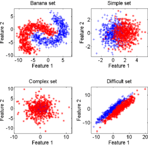
Figure 4.1.1 – Outputs of the various artificial data generators 4.2 COMBINED CLASSIFIERS
Combination performance is evaluated using the following 6 classifiers:
- QBNC: Quadratic Bayesian Normal classifier with one kernel per class (Bayes-Normal-2);
- FLSLC: Fisher Linear Least Squares Classifier;
- NMC: Nearest Mean Classifier;
- KNNC: nearest neighbor classifier;
- ParzenC: Parzen classifier;
- BayesN: Naive Bayesian classifier.
Each of these classifiers was first trained and tested on all the datasets in order to evaluate their overall performance. The training and test sets were constructed by bootstrapping[20] from the original data, with zero intersection between the 2 datasets each time.
Bootstrapping is generally useful for estimating the distribution of a statistic (mean, variance, etc.). Among the various methods available is the Monte Carlo algorithm [25] for simple resampling. The idea is to make an initial measurement of the desired statistic on the available dataset, then randomly sample (with discount) this dataset and repeat the measurement. This method is repeated until acceptable precision is achieved.
The KNNC, ParzenC and NMC classifiers are adaptive: the value of their parameters (i.e.
for KNNC and ParzenC) is optimized during the learning phase. Then, once the parameter has been set, it is not called into question during recognition. 4.3 COMBINATION METHODS
We choose to test the different combinations according to the different ways of calculating local accuracy:
- LAO: a priori local accuracy according to [36] (equation 3.2.3.2) ;
- a posteriori local accuracy according to [36] (equation 3.2.3.3);
- LAP: Didaci’s method [3] (equation 3.2.3.4);
- LAS: the method proposed in equation 3.2.3.6.
The LAO, LCA and LAS methods have also been compared using Giacinto’s similarity constraint (MCB approach)[16][11]. For these tests, we evolve the neighborhood size (
) to test its influence on the results. We set the maximum value of lower than the total number of individuals, in order to remain in the case of local, and not global, accuracy analysis. For the results presented below, we use the legend of figure ??. To situate the results in terms of computing time, it should be noted that all tests are run on a computer equipped with an AMD Athlon XP2600+ with 1GB RAM running Ubuntu 7.x.
5 DISCUSSION
5.1 DIRECT APPROACHES
An analysis of the behavior of the Banana and Difficult datasets (figures 5.2.1 and 5.2.2) gives an initial idea of the behavior of the accuracy measures. For the Banana dataset, the a posteriori accuracy measure (LCA) is the only one that increases as a function of neighborhood size. In this case, increasing the size of the neighborhood (
) increases the ratio between the number of well-ranked individuals and the number of recognized individuals. For the Difficult dataset (figure 5.2.2), it’s the LAP method that increases slightly with . Here, the increase in is weighted by the distance to the individual to be recognized, to improve the accuracy measure. In all other cases, accuracy is at best roughly stable and at worst decreases slightly with increasing neighborhood size. 5.2 NEIGHBORHOOD LIMITATION APPROACHES
With regard to the results obtained with artificial datasets (figures 5.2.1 and 5.2.2), we note the significant variation in performance for the LAO, LCA and LAP methods (with or without MCB), compared with the results obtained with natural datasets (figures 5.2.3, 5.2.4 and 5.2.5). The LAO and LCA methods take into account the number of well-ranked individuals in the neighborhood, but as the neighborhood grows, the performance tends towards that of the most efficient classifier on its own, which we note by integrating the performance of the classifiers alone (tables 5.3.1 and 5.3.3) in the figures below. If, on the other hand, we take natural data, whose distribution density is lower (individuals are better distributed in the attribute space), then a statistical approach is more representative of overall behavior (and not the best classifier). As the probability laws are unknown, we measure the distribution of individuals according to 2 criteria: the mean Euclidean distance
 between individuals, and its standard deviation
  . The data are presented in Table 5.2.1. The greater the mean distance and standard deviation, the less influence the size of the DCS neighborhood has on overall performance. It’s also interesting to note that the LAS method (with or without MCB) seems the least sensitive to neighborhood size, except of course for the fact that the larger is, the poorer the overall performance (as it tends towards the overall performance of the best classifier on its own).
 Note in table 5.2.1 that for artificial data (Banana, Complex, Difficult and Simple) the means and standard deviations are of the same order, for a dimension fixed at 2. This is not the case for natural data, for which the ratios between mean distances and standard deviations indicate the very high complexity of these databases.
data 
dimension Wisconsin breast cancer 

10 Pima Indians diabetes 

8 German 

24 Ionosphere 

34 Sonar 

60 Banana set 

2 Complex set 

2 Difficult set 

2 Simple set 

2 Table 5.2.1 – Average distance and standard deviation between individuals 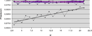
Figure 5.2.1 – Influence of neighborhood size (Banana dataset) 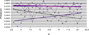
Figure 5.2.2 – Influence of neighborhood size (Difficult dataset) 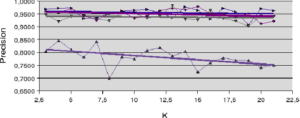
Figure 5.2.3 – Influence of neighborhood size (Ionosphere dataset) 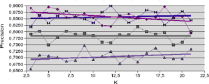
Figure 5.2.4 – Diabete 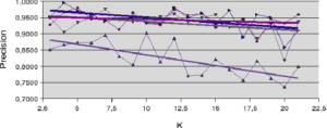
Figure 5.2.5 – Sonar 
Figure 5.2.6 – Legend 5.3 THE CONTRIBUTION OF MULTIPLE CLASSIFIER BEHAVIOR (MCB)
The
nearest neighbors of a test individual are first identified in the training dataset. Those characterized by MCBs “similar” (equation 3.2.2.1) to those of unknown individuals (from the test set) are then selected to calculate local accuracies and perform dynamic selection. Tables 5.3.1 and 5.3.3 show the best performance for each classifier alone, then for each DCS method (for all
). Note first (5.3.3), the performance gain brought by the MCB to the LAO and LCA methods. These results are in line with Huang’s remarks in [16]. Secondly, the results of the LAS method are degraded when combined with the MCB approach. Indeed, the LAS method, based on an average calculation, requires a maximum of information about the neighborhood, whereas the MCB does not take into account the closest individuals in terms of distance, but only those in terms of classifier response. So, for each method of calculating overall accuracy, the MCB improves the probability of taking the individuals for whom the system presents the best certainty (which can be likened to a measure of credibility in evidence theory), except for our approach, which doesn’t need it. Thus, MCB improves performance by selecting information according to the similarity of the classifiers’ outputs. However, there is an exception for methods that take into account the distances between known individuals and the query individual . We also studied the behavior of a group of classifiers constructed a priori by diversity optimization. The measure used is entropy, and we selected, for each dataset, the association of classifiers with the highest entropy. The rate of correct classification obtained is shown in table 5.3.2.
We observe here that the diversity-based method of constructing a set of classifiers does not improve the overall results obtained by the classifiers alone. This suggests that this method is not suitable for dynamic construction of classifier sets, compared with static a priori construction.
Banana Complex Difficult Simple Diabetes Sonar German Cancer Ionosphere Quadratic 0.87 0.83 0.96 0.86 0.71 0.81 0.74 0.96 0.92 Pseudo Fisher 0.87 0.47 0.96 0.86 0.72 0.84 0.69 0.95 0.85 Nearest Mean 0.82 0.47 0.72 0.86 0.59 0.70 0.58 0.52 0.76 KNN 0.99 0.93 0.97 0.93 0.86 0.92 0.86 0.84 0.94 Parzen 0.99 0.88 0.95 0.89 0.74 0.92 0.63 0.51 0.92 Naive Bayesian 0.94 0.80 0.69 0.85 0.74 0.88 0.68 0.98 0.50 Best Performance 0.99 0.93 0.97 0.93 0.86 0.92 0.86 0.98 0.94 Table 5.3.1 – Best performance for each classifier alone Banana Complex Difficult Simple Diabetes Sonar German Cancer Ionosphere Entropy measurement 0.99 0.58 0.91 0.87 0.76 0.80 0.74 0.67 0.90 Table 5.3.2 – Best performance by combination built on diversity Banana Complex Difficult Simple Diabetes Sonar German Cancer Ionosphere LAO 1.00 0.93 0.98 0.95 0.90 0.98 0.89 0.98 0.98 LAO+MCB 1.00 0.94 0.98 0.95 0.90 0.99 0.90 0.99 0.99 LCA 0.96 0.91 0.97 0.91 0.82 0.97 0.85 0.97 0.98 LCA+MCB 1.00 0.95 0.98 0.96 0.89 1.00 0.89 0.99 0.99 LAP 0.99 0.86 0.97 0.87 0.75 0.90 0.65 0.65 0.85 LAS 1.00 0.95 0.99 0.95 0.90 0.99 0.92 0.99 0.98 LAS+MCB 0.94 0.90 0.98 0.93 0.83 0.96 0.85 0.99 0.99 Best Performance 1.00 0.95 0.99 0.96 0.90 1.00 0.92 0.99 0.99 Table 5.3.3 – Best performance for each method tested 5.4 THE BENEFITS OF DYNAMIC COMBINATION
The results obtained by a priori static combination of classifiers through diversity optimization are very poor, compared with classifiers alone or dynamically combined, for the “Complex” or “Breast Cancer Wisconsin” data. This behavior can be explained by the fact that diversity is a criterion based on the global behavior that compares a classifier to the group, whereas local accuracy is a criterion based on the distribution of individuals in the attribute space.
Finally, for the datasets tested, the results given by DCS are always better than those obtained by the best classifier alone (tables 5.3.1 and 5.3.3).
The LCA+MCB and LAS methods even give the best overall recognition rate (table 5.3.3) for a similar computation time (around 80ms per individual for artificial data on an AMD Athlon XP2600+ with 1GB RAM under Ubuntu 7.x). The expected benefits of dynamic classifier selection are for very large databases, it is then possible to implement only a few classifiers, certainly not the best in terms of performance, but at least the best in terms of computation time. In this way, computation time is greatly improved compared with a single, overly complex classifier. This is particularly interesting in view of the growth in data mining techniques [6], where ever-faster response times are expected, while ever-greater quantities of data need to be managed.
However, for the sake of completeness, we must take into account the most important cost of the method, which is related to a neighborhood search on the training set. A practical implementation of the method would see a great gain here in using optimized approaches and organizing the training set in tree form, for example.
6 CONCLUSION
Two ideas are presented here. The first is the measurement of local accuracy for classification. The second is the use of local accuracy in dynamic classifier systems (DCS). We have shown the improvement brought about by these ideas, compared to the a priori use of a single classifier. We also explained the importance of using a small neighborhood size when calculating the local accuracy of a classifier (local accuracy tends towards global accuracy as the size of the neighborhood increases). Finally, we proposed a different way of calculating local accuracy, which gives results as good as those given by the best of existing methods, but with lower algorithmic complexity.
It is possible to develop other methods for measuring local accuracy using knowledge about the classifiers, especially using the position of unknown individuals relative to class boundaries and centers. This adaptation to the configuration is close to that of the Support Vector Machine (SVM) principle [30].
However, with this kind of approach, a few precautions need to be taken with the constraints imposed by natural data (i.e. zeros on the variance/covariance matrices).
We show here the interest of using information on the distribution of individuals in the attribute space, especially in a given neighborhood, using an L1 distance to calculate local accuracy. The next step in this work could be to exploit the shape of the neighborhood, using the information carried by the covariance between individuals (variance/covariance matrices, eigenvalues), with the idea of creating an adaptive metric as shown in [14]. This kind of metric reduces the neighborhood in directions along which the class centers differ, with the intention of ending up on a neighborhood for which the class centers coincide (and thus have the closest neighborhood suitable for classification).
Nevertheless, measuring accuracy is the most interesting aspect of an information processing chain [7][6]. With the ability to assess the quality of the decision, the system has the information to feed back into dynamic operator execution and decision-making [32].
If we return to the problem of integrating precision for decision-making, we’ve just seen how to calculate this precision for classifiers, and how to use it to dynamically choose a classifier, a priori the best suited to handle the unknown individual being analyzed.
REFERENCES
[1] C. Conversano, R. Siciliano, and F. Mola. Supervised classifier combination through generalized additive multi-model. In MCS ’00: Proceedings of the First InternationalWorkshop on Multiple Classifier Systems, pages 167-176, London, UK, 2000. Springer-Verlag.
[2] L. P. Cordella, P. Foggia, C. Sansone, F. Tortorella, and M. Vento. A cascaded multiple expert system for verification. In MCS ’00: Proceedings of the First International Workshop on Multiple Classifier Systems, pages 330-339, London, UK, 2000. Springer-Verlag.
[3] L. Didaci, G. Giacinto, F. Roli, and G. L. Marcialis. A study on the performances of dynamic classifier selection based on local accuracy estimation. Pattern Recognition, 38 :2188-2191, 2005.
[4] T. G. Dietterich. Approximate statistical tests for comparing supervised classification learning algorithms. Neural Computation, 7(10) :1895-1942, 1998.
[5] R. P.W. Duin and D. M. J. Tax. Experiments with classifier combining rules. In MCS ’00: Proceedings of the First International Workshop on Multiple Classifier Systems, pages 16-29, London, UK, 2000. Springer-Verlag.
[6] U. Fayyad, G. Pietetsky-Shapiro, and P. Smyth. From data mining to knowledge discovery in databases. AI Magazine, 17(3) :37-54, 1996.
[7] U. Fayyad, G. Pietetsky-Shapiro, and P. Smyth. Knowledge discovery and data mining: towards a unifying framework. Proceedings of the 2nd International Conference on Knowledge Discovery and Data Mining, pages 82-88, 1996.
[8] J. L. Fleiss. Statistical Methods for Rates and Proportions. John Wiley & Sons, 1981.
[9] J. Ghosh. Multiclassifier systems: Back to the future. In MCS ’02: Proceedings of the Third International Workshop on Multiple Classifier Systems, pages 1-15, London, UK, 2002. Springer-Verlag.
[10] G. Giacinto and F. Roli. Adaptive selection of image classifiers. ICIAP ’97, Lecture Notes in Computer Science, 1310 :38-45, 1997.
[11] G. Giacinto and F. Roli. Dynamic classifier selection based on multiple classifier behavior. Pattern Recognition, 34 :1879-1881, 2001.
[12] G. Giacinto, F. Roli, and G. Fumera. Selection of image classifiers. Electronics Letters, 36(5) :420-422, 2000.
[13] D. J. Hand, N. M. Adams, and M. G. Kelly. Multiple classifier systems based on interpretable linear classifiers. In MCS ’01: Proceedings of the Second International Workshop on Multiple Classifier Systems, pages 136-147, London, UK, 2001. Springer-Verlag.
[14] T. Hastie and R. Tibshirani. Discriminant adaptive nearest neighbor classification. IEEE Transaction on Pattern Analysis and Machine Intelligence, 18(6) :607-616, 1996.
[15] T. K. Ho. Complexity of classification problems and comparative advantages of combined classifiers. In MCS ’00: Proceedings of the First International Workshop on Multiple Classifier Systems, pages 97-106, London, UK, 2000. Springer-Verlag.
[16] Y. S. Huang and C. Y. Suen. A method of combining multiple experts for the recognition of unconstrained handwritten numerals. IEEE Trans. on Pattern Analysis and Machine Intelligence 17 :90-94, 1995.
[17] K. G. Ianakiev and V. Govindaraju. Architecture for classifier combination using entropy measures. In MCS ’00: Proceedings of the First International Workshop on Multiple Classifier Systems, pages 340-350, London, UK, 2000. Springer-Verlag.
[18] L. I. Kuncheva. Switching between selection and fusion in combining classifiers: an experiment. IEEE Trans. Syst. Man. Cybernet. Part B 32 2002.
[19] L. I. Kuncheva. Combining Pattern Classifiers. Wiley, 2004.
[20] L. I. Kuncheva, M. Skurichina, and R.P.W. Duin. An experimental study on diversity for bagging and boosting with linear classifiers. Information fusion, pages 245-258, 2002.
[21] P. Latinne, O. Debeir, and C. Decaestecker. Different ways of weakening decision trees and their impact on classification accuracy of dt combination. In MCS ’00: Proceedings of the First International Workshop on Multiple Classifier Systems, pages 200-209, London, UK, 2000. Springer-Verlag.
[22] L. Lebart, A. Morineau, and M. Piron. Multidimensional exploratory statistics. DUNOD, 1995.
[23] S.W. Looney. A statistical technique for comparing the accuracies of several classifiers. Pattern Recognition Letters, 8(1) :5-9, 19988.
[24] S. P. Luttrell. A self-organising approach to multiple classifier fusion. In MCS ’01: Proceedings of the Second International Workshop on Multiple Classifier Systems, pages 319-328, London, UK, 2001. Springer-Verlag.
[25] N. Metropolis. The beginning of the monte carlo method. Los Alamos Science, 15 :125-130, 1987.
[26] J. Parker. Rank and response combination from confusion matrix data. Information Fusion, 2 :113-120, 2001.
[27] F. Roli, G. Fumera, and J. Kittler. Fixed and trained combiners for fusion of imbalanced pattern classifiers. 5th International Conference on Information Fusion, pages 278-284, 2002.
[28] F. Roli, G. Giacinto, and G. Vernazza. Methods for designing multiple classifier systems. In MCS ’01: Proceedings of the Second International Workshop on Multiple Classifier Systems, pages 78-87, London, UK, 2001. Springer-Verlag.
[29] J. W. Jr Sammon. A nonlinear mapping for data structure analysis. IEEE Transactions on Computers, 18 :401-409, 1969.
[30] J. Shawe-Taylor and N. Cristianini. Support Vector Machines and other kernel-based learning methods. Cambridge University Press, 2000.
[31] M. Skurichina, L. I. Kuncheva, and R. P.W. Duin. Bagging and boosting for the nearest mean classifier: Effects of sample size on diversity and accuracy. In MCS ’02: Proceedings of the Third International Workshop on Multiple Classifier Systems, pages 62-71, London, UK, 2002. Springer-Verlag.
[32] S. Sochacki, N. Richard, and P. Bouyer. A comparative study of different statistical moments using an accuracy criterion. In Seventh IAPR International Workshop on Graphics Recognition – GREC 2007, September 2007.
[33] D. M. J. Tax and R. P. W. Duin. Combining one-class classifiers. In MCS ’01: Proceedings of the Second International Workshop on Multiple Classifier Systems, pages 299-308, London, UK, 2001. Springer-Verlag.
[34] P. Viola and M. Jones. Rapid object detection using a boosted cascade of simple features. In IEEE Conference on Computer Vision and Pattern Recognition (CVPR01), volume 1, pages 511-518, Kaui(Hawaii), December 2001.
[35] M. S. Wong and W. Y. Yan. Investigation of diversity and accuracy in ensemble of classifiers using bayesian decision rules. In International Workshop on Earth Observation and Remote Sensing Applications (EORSA 2008), pages 1-6, 2008.
[36] K. Woods, W. P. Kegelmeyer, and K. Bowyer. Combination of multiple classifiers using local accuracy estimates. IEEE Trans. on Pattern Analysis and Machine Intelligence 19 :405-410, 1997.
[37] L. Xu and A. Krzyzakand C. Y. Suen. Methods for combining multiple classifiers and their applications to handwriting recognition. IEEE Transactions on Systems, Man and Cybernetics, 22(3) :418-435, 1992.
[38] H. Khoufi Zouari. Contribution à l’évaluation des méthodes de combinaison parallèle de classifieurs par simulation. PhD thesis, Université de Rouen, December 2004. - Local accuracy a priori
 http://www.diee.unica.it/mcs/previous-mcs.html