How to decide in the presence of imprecision?

S. Sochacki, PhD in Computer Science

A2D, ZA Les Minimes, 1 rue de la Trinquette, 17000 La Rochelle, FRANCE

1 Introduction

Imprecision/uncertainty/conflict
AI Act, explainability

How do you decide in IT? What does an automatic system base its decisions on? Very often, this kind of system is based on a principle of decision rules (often probabilistic), or on a pignistic approach (a level entirely dedicated to decision-making and clearly separated from data modeling).

Although a very large proportion of image processing applications for the general public are geared towards the enhancement, restoration or processing of photographs, in an industrial context, the target applications are image-based decision-making. While the classes of information used for this purpose are well known (texture, shape, color), they are not all of the same interest in decision support. Various forms of learning have therefore been developed to identify the best possible combination of information. Dozens of solutions exist to answer this question, and some even combine several of these approaches to optimize decision-making as much as possible.

However, while not all information classes, and more specifically all information extraction operators (Zernike moments, D’Haralick attributes, to name but two), are of equal interest for decision-making purposes, the information extracted is judged to be of equal quality. And yet, image processing comes in part from signal processing, and thus from the world of physics and, more specifically, metrology. So we’re a long way from a binary world, where information is true or false, but certain as to its assignment. In metrology, measurement only exists in relation to a criterion of precision or tolerance. This criterion quantifies the range of values within which the measurement lies with a good degree of certainty. This point of view, typical of needle-based metrology, is often forgotten in the transition to digital technology. And yet, every scientist remains sceptical when announcing a result with more than 3 digits behind the decimal point (when this precision has not been justified beforehand).

A2D is committed to developing applications using decision-making algorithms to meet these new needs, while respecting the constraints linked to trusted AI (AI Act , ISO/IEC 42001 ) and energy sobriety. In practice, we are designing data processing and analysis applications to understand outdoor scenes, digitized with a view to detecting precise areas of interest, depending on business uses.

We also endeavor to provide, at all times during the processing of information, an explanation of the results obtained and the choices proposed by the machine.

2 Probabilistic approach

Since our aim is to propose a new extension to decision-making tools, we felt it was important to stay within the framework of mathematically-based tools, as opposed to rule-based tools. As probabilities are at the heart of these approaches, we have chosen to start this study from this formalism.

Classically, we call probability the evaluation of the likelihood of an event. It is represented by a real number between 0 and 1, indicating the degree of risk (or chance) that the event will occur. In the typical example of a coin toss, the event “tails side up” has a probability of , which means that after tossing the coin a very large number of times, the frequency of occurrence of “tails side up” will be .

In probability, an event can be just about anything you can imagine, whether it happens or not. It could be that the weather will be fine tomorrow, or that a roll of a die will produce the number 6. The only constraint is to be able to verify the event; it’s perfectly possible to check whether the weather will be fine tomorrow (an event that we measure personally, the following day, according to our tastes in terms of sunshine, temperature, etc.), or whether we manage to obtain the number 6 with a die.

We’ll say that an event with a probability of 0 is impossible, while an event with a probability of 1 is certain.

Note that probability is a tool for predicting real-world events, not for explaining them. It’s about studying sets by measuring them.

2.1 Definitions

An experiment is said to be random when its outcome cannot be predicted. Let’s define , a random experiment whose result is an element of , the set of all possible outcomes, called the universe of possibilities or frame of reference.

Let be theset of parts of . An event is then a logical proposition linked to an experiment, relative to its result.

Let be the set of events and subset of . For all and :

• A \cup BAB denotes the realization of and .
• denotes the opposite of .
• is the certain event
• is the impossible event

When the reference frame is finite, designates all the parts of , usually noted . When the reference frame is (or an interval of ), the notion of tribe makes it possible to define :

• \mathcal{A}\subseteq\mathcal{P}(\Omega)\emptyset\in\mathcal{A}\forall\{A_1,\ldots,A_n\}\in\mathcal{A}\bigcup_iA_i\in\mathcal{A}\bigcap_iA_i\in\mathcal{A}\bar{A}\in\mathcal{A}\forall A\in\mathcal{A}(\Omega,\mathcal{A})\mathcal{A}[0,1]1
• For all incompatible elements and (i.e. ), .

The number quantifies how likely the event is.

In the case of a throw of the dice, we can state that represents all 6 faces of the dice. Thus, the probability of obtaining a number between 1 and 6 is certain, and therefore equal to 1. We’ll write .

Similarly, the probability of obtaining 1 (or 2, or 3, or 4 etc.) is 1/6. So, .

Related to , in the case where is finite, a probability distribution is defined as a function of in , such that:

(2.1.1)  

with the normalization condition:

(2.1.2)  

Note that .

2.2 Bayes’ rule

The introduction of a statistical model leads to a decision theory directly applicable, in principle, to the problem of classification. This application is essentially based on Bayes’ rule, which makes it possible to evaluate probabilities a posteriori (i.e. after the actual observation of certain quantities) knowing the conditional probability distributions a priori (i.e. independent of any constraints on the observed variables). The probabilities required to make a decision according to Bayes’ rule are provided by one (or more) statistical classifiers, which indicate the probability of a given individual belonging to each class of the problem.

In probability theory, Bayes’ theorem states conditional probabilities: given two events and , Bayes’ theorem allows us to determine the probability of knowing , if we know the probabilities: of , of and of knowing A. To arrive at Bayes’ theorem, we need to start from one of the definitions of conditional probability: , noting the probability that and will both occur. Dividing on both sides by , we obtain , i.e. Bayes’ theorem. Each term in Bayes’ theorem has a common name. The term is the a priori probability of A. It is “prior” in the sense that it precedes any information about . is also called the marginal probability of . The term is called the a posteriori probability of knowing (or of under condition ). It is “posterior”, in the sense that it depends directly on . The term , for a known , is called the likelihood function of . Similarly, the term is called the marginal or a priori probability of .

But, as previously stated, the probability values used by Bayes’ rule are provided by statistical classifiers, or simply by estimating the probability distributions of each class.

2.3 Statistical decision-making

From the hypothesis about the probability distributions of the problem’s classes (and its validation tests) to the measurement of the distance to the center of each class, via various forms of model estimation, there are a huge number of methods in the field of statistics. Our aim is not to make an exhaustive study of them, but to compare theories (statistics, decision theory…) on the principle.

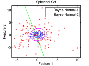
Let’s just say that there are two main types of statistical approach: linear classifiers and quadratic classifiers. The former are so called because their approach consists of partitioning the attribute space in a simple way, based on straight lines, each straight line symbolizing the boundary between two classes, as illustrated by the boundary in green in figure 2.3.1. The second approach is more complex, as it attempts to estimate the shape of the boundaries between regions, thus obtaining the circular separation between classes.

2.3.1 Bayesian classifier [93][4][14]

Bayes decision theory is a statistical approach to the problem. It is based on the following assumptions:

• The decision problem is expressed in terms of probabilities
• The value of the a priori probabilities of drawing a class is known

Let be a random variable representing the individual’s state ( if the individual belongs to class ).

Let be the set of possible states or classes of a problem.

The set of a priori probabilities is calculated from observations made on the system under study. In the absence of other information, we have no choice but to write individual . But if it is possible to obtain other information (measurements), then , the probability density of knowing that the individual is , or the probability density conditional on his belonging to , can be calculated.

p(\omega_j)\omega_jp(\omega_j|x)x\omega_jx=\{x_1 \ldots x_d\}{mathbb{R}}^dx\omega_j

Sp(x)x\omega_jp(\omega_j)\omega_jp(\omega_j|x)=max_{i=1,n}(p(\omega_i|x))A={alpha_1,\ldots,\alpha_k\}aX_1, X_2, …, X_n\mu\sigma^2\bar{X}=\frac {1}{n}\sum_{i=1}^{n}X_id>0

n\geq 30X_1+X_2+…+X_n

(2.3.1.6)  

xN(\bar whose probability density will be expressed in matrix form:

(2.3.1.7)  

with mean of a class, covariance matrix of class and determinant of covariance matrix of class .

The conditional probability is therefore expressed by the following equation:

(2.3.1.8)  

The classification operation consists in calculating for each measure its probability of belonging to all the classes, and assigning it to the class that verifies the maximum a posteriori probability.

2.3.2 K-nearest neighbors (KPPV or KNN)

This approach consists in taking a given number () of known individuals from the attribute space, individuals chosen from the neighborhood of the individual whose class we’re trying to estimate. The labeling of the unknown individual is based on knowledge of the classes represented in this neighborhood.

The k-nearest neighbor rule was formalized by Fix and Hodges [5] in the 1950s. This rule consists in basing the choice of the neighborhood on the number of observations it contains, fixed at among the total number of observations . In other words, we select a subset of individuals from the set of observations. It is the volume of that is variable. The probability density estimator is then expressed as follows:

(2.3.2.1)  

The first assumption corresponds to a space completely occupied by observations: when the number of observations is infinite, these observations occupy the space uniformly. The second hypothesis considers that, for an infinite number of observations, any subset of cardinal is occupied by an infinite number of uniformly distributed elements.

In the context of supervised classification, the conditional probability distribution can be approximated by:

(2.3.2.2)  

where is the number of observations contained in the volume belonging to the label class and the total number of observations belonging to the class . The a posteriori law of observation of a label conditional on an observation is obtained with Bayes’ rule:

(2.3.2.3)  

The choice of is linked to the learning base. Choosing a large allows local properties to be exploited to the full, but requires a large number of samples to keep the neighborhood volume small. Often, is chosen as the square root of the average number of elements per class, i.e. [2].

2.4 Summary

But how do you choose anything other than what is statistically most likely?

The problem then arises of measuring the accuracy of a decision and producing a measure of accuracy, even if the problem may be this measure.

3 Theory of evidence

The transferable belief model (TBM) is a generic formal framework developed by Philippe Smets [20] for the representation and combination of knowledge. TBM is based on the definition of belief functions provided by information sources that may be complementary, redundant and possibly non-independent. It proposes a set of operators for combining these functions. It is therefore naturally used in the context of information fusion to improve the analysis and interpretation of data from multiple information sources. This framework naturally corresponds to the one we’re concerned with in its decision-making aspect, thanks to different information from different attributes.

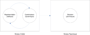
One of the fundamental features of TBM is the differentiation between the knowledge representation and decision levels. This differentiation is much less preponderant in other approaches, particularly the probabilistic model, where decision is often the sole objective. TBM’s reasoning mechanisms are therefore grouped into two levels, as illustrated in figure 3.1 :

• The credal level: home to knowledge representation (static part), combinations and reasoning about this knowledge (dynamic part).
• The pignistic level indicates a decision, possibly taking into account the risk and/or reward associated with that decision.

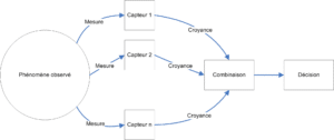
In the context of representation in the form of a processing chain, we are faced with the problem of observing the same event from several sources, and combining the information provided by these sources (see Figure 3.2), which raises the following questions:

• How can we represent the knowledge of an information source in the form of belief functions, and what advantages can we derive from such a representation?
• How can we combine several sources of belief functions to summarize information and improve decision-making?
• How to make a decision based on belief functions?

3.1 Presentation

Let’s take the example of handwritten number recognition. The possible digits that can be written are called hypotheses, and the set of hypotheses forms the discernment frame, usually denoted . For our example, where is the symbol representing the digit . Since two hypotheses can’t be true simultaneously (a symbol representing several digits can’t be written at the same time), they are assumed to be exclusive, resulting in a null intersection between them (i.e. ). Now let’s suppose that the document we’re studying is degraded, or that the figure is very badly written, a reader would then give a weighted opinion on this figure, making it a source of information. With his available knowledge, the reader would say that it’s either , or . The question is how to represent this information.

In the context of probability theory, the answer is given by the principle of equiprobability, i.e. each digit is assigned the same probability () so that the sum of all probabilities is equal to 1. Thus, the probability distribution for this digit is equal to:

This probability is only assigned to hypotheses taken alone (also called singletons).

In evidence theory, the main notion is that of belief functions, within which knowledge is modeled by a distribution of belief masses. In our example, the entire belief mass (an integer unit, as with probabilities) is assigned to the union of all hypotheses, i.e. the proposition :

As we can see, this mass gives us no information about the belief of each of the hypotheses (, and ) that make it up. We can then say that the belief mass explicitly models doubt (or ignorance) about this set of hypotheses. To return to probability theory, the value of the probability on a union of hypotheses is implicitly derived from the probability on the singletons, a probability established from the sum of all the private probabilities of the common part, i.e. the probability of the intersection. For example:

Here, the probability on represents the common part of the events“The number is 1” and“The number is 7“, which we need to remove so as not to count the events twice. In the case where the hypotheses are exclusive (a case we’ll come back to throughout this article), we obtain :

taking into account that by definition.

Unlike probabilities, a mass function on a union of hypotheses is not equal to the sum of the masses of the hypotheses making up the union [10], and it is precisely thanks to this property that we represent doubt between hypotheses. Moreover, belief functions have the advantage of being generic, since they are the mathematical representation of a superset of probability functions. Indeed, a mass distribution, where only singleton hypotheses have non-zero mass, can be interpreted as a probability distribution. Klir and Wierman explain in [10] that belief functions mathematically generalize possibility functions, and that each of these functions (probabilities, possibilities and beliefs) has particular characteristics and enables knowledge to be modeled differently.

Let’s now look at the mathematical formalism of belief functions, based on the models of Dempster [6][7], Shafer [15], transferable beliefs [20] and the Hints model [9]. For this work, we have restricted ourselves to the axiomatized and formalized framework of the transferable belief model developed by P. Smets.

3.2 Formalism

3.2.1 Introduction

If we return to the problem of managing multiple sources of information (as illustrated in Figure 3.2), what we’re trying to do is determine the actual state of the system under study, using multiple observations from multiple observers. In our case, will be the decision to be produced and the various attributes provide the observations on the system.

We assume that this state takes discrete values (the hypotheses) and that the set of possible hypotheses is called the discernment frame (or \textbf{universe of discourse}), generally noted:

(3.2.1.1)  

The total number of hypotheses making up is called the cardinal and is written as . As we saw earlier, all hypotheses are considered exclusive.

The system’s set of observers (the sensors in figure 3.2) provides a weighted opinion, represented by a belief function, about its actual state . We call these sensors belief sources.

3.2.2 Mass functions

Let be the space formed by all the parts of , i.e. the space containing all the possible subsets formed by the hypotheses and unions of hypotheses, i.e. :

Let be a proposition such that , e.g. . explicitly represents the doubt between its hypotheses ( and ). As we saw above, belief masses are non-additive, which is a fundamental difference from probability theory. Thus, the belief mass allocated to gives no information about the hypotheses and subsets making up [10].

We can define a distribution of belief masses (BBA: basic belief assignment) as a set of belief masses concerning any propositions verifying:

(3.2.2.1)  

Each of the sensors observing the system will contribute its own mass distribution.

The mass supplied by a sensor is that sensor’s share of belief in the proposition ““, where is the actual state of the observed system. Any non-zero mass element (i.e. ) is called the focal element of the belief mass distribution. Ramasso [13] presents a notable set of belief mass distributions in his dissertation.

When the universe of discourse contains all possible hypotheses (i.e. when it is exhaustive), it necessarily contains the hypothesis that describes the observed system. Otherwise, the discernment framework is not adapted to the problem at hand.

From the moment is exhaustive, the mass of the empty set is zero (), the mass is said to be normal, and the problem then enters the framework of a closed world as in the case of Shafer’s model [15].

In the case of the transferable belief model, the universe of discourse can be non-exhaustive; the mass of the set is non-zero () and is said to be subnormal, and in this case the problematic is part of an open-world framework. This type of construction makes it possible to redefine the discernment framework, for example, by adding a hypothesis based on the mass of the empty set, such as a rejection hypothesis. Rejection hypotheses correspond to states such as“I don’t know“. At the end of the chain, they allow us to reject an individual for whom there is too much doubt, rather than taking the risk of classifying him or her in spite of everything. To move from an open to a closed world, we need to redistribute the mass of the empty set to the other subsets of the space [11].

To summarize what we’ve seen so far, the mass function is determined a priori, without the need for probabilistic considerations. It may correspond to an observer’s subjective attribution of degrees of credibility to the realization of various conceivable events on .

The assignment of values is used to express the degree to which the expert or observer judges that each hypothesis is likely to come true. Thus, describes its imprecision relative to these degrees.

3.2.3 Dempster’s combination rule

If we return to figure 3.2, we see that the problem at hand is information fusion, i.e. combining heterogeneous information from several sources to improve decision-making [3].

Let’s now look at a formal tool developed within the framework of the transferable belief model for information fusion. We assume that the sources are distinct [16][21][22][23], by analogy with theindependence of random variables in statistics.

It may happen that for the same hypothesis, two sensors provide completely different information. From a formal point of view, when combining two belief mass functions and , the intersection between the focal elements may be empty. The resulting belief mass function in this combination will be non-zero on the empty set. This value then quantifies the discordance between the belief sources, and is called conflict [17]. A normalization can be performed, bringing the conjunctive combination rule back to Dempster’s orthogonal rule [6][7] (denoted ) used in Shafer’s model [15][18]:
\begin {eqnarray}
m_{1\oplus 2}(A)=(m_1 \oplus m_2)(A)=\left\{
\begin{array}{lccc}
\frac{m_{1\overlay{\cap}{\bigcirc}2}(A)}{1-m_{1\overlay{\cap}{\bigcirc}2}(\emptyset)}, & \forall A\subseteq\Omega & \mathrm{si }&A\neq\emptyset\\\
0 & & \mathrm{si }&A=\emptyset\\
\end{array}
\right.
\label{incertitude:eq:dempsterrule}\tag{3.2.3.1}
\end{eqnarray}
Another way of writing this combination rule is:

*** QuickLaTeX cannot compile formula:
\begin{eqnarray*}
m(A)=\frac{{sum_{B\cap C=A}m_1(B)m_2(C)}{{sum_{B\cap Cneq0}m_1(B)m_2(C)} & \forall A\subseteq\Omega
\end{eqnarray*}

*** Error message:
File ended while scanning use of \frac .
Emergency stop.

With, as a measure of the conflict between sources:

(3.2.3.3)  

3.2.4 Simple attenuation

The simple weakening rule to incorporate source reliability. Applying the disjunctive combination rule can be too conservative when the sources of belief mass functions are unreliable. It can thus lead to a completely non-informative (empty) belief mass function. In some applications, however, it is possible to quantify reliability, enabling a less conservative combination rule to be applied in the case of unreliable sources.

Taking reliability into account in the context of belief functions is calledweakening, because the process consists in weighting the mass of elements of a belief mass function. The first work on weakening in the context of belief functions was developed by Shafer [15], axiomatized by Smets [16] and generalized by Mercier and Denœux [12]. Generalized weakening was called contextual weakening.

Shafer’s simple weakening of a belief mass function is defined as the weighting of each mass of the distribution by a coefficient called reliability and where is the rate of weakening.

Formally:

(3.2.4.1)  

By the principle of minimum information (maximum entropy), the rest of the mass (after weighting) is transferred to the element of ignorance . The more reliable the source (and the lower the rate of weakening ), the less the belief mass function is modified, whereas as reliability decreases, the belief mass function resulting from weakening tends towards the empty belief mass function.

3.3 The pignistic decision

From the set of belief functions provided by all the sensors, and following their combination by Dempster’s rule, we obtain a unique belief function for each of the possible hypotheses modeling the system’s knowledge. This knowledge is then used to make a decision on one of the hypotheses.

Note that the system’s hypotheses don’t necessarily represent the only possible classes (i.e. the 26 letters of our alphabet). It is also possible to create a new hypothesis corresponding to the event “none of the known hypotheses”. This is referred to as rejection, i.e. the unknown individual is not re-injected into the chain, but simply classified as “impossible to recognize”. The measure of sensor conflict during the Dempster merge (see equation 3.2.3.3) is also a measure on which the system can base its rejection of the individual.

Information fusion systems, whether based on probability theory, possibility theory or belief functions, are designed for decision making and decision analysis. Decision-making consists in choosing a hypothesis on a betting framework, generally the discernment framework. Decision-making can be automatic or left to the responsibility of the end-user (as in the case of diagnostic aids in the field of medicine).

Within the framework of the transferable belief model, the decision phase is based on the pignistic probability distribution noted from the mass distribution [19]. The pignistic transform consists of distributing the mass of a proposition equiprobably over the hypotheses contained in .

Formally:

(3.3.1)  

where is given by:

(3.3.2)  

The decision is generally made by choosing the element with the highest pignistic probability:

(3.3.3)  

The agent who relies on the pignistic transform in the decision-making phase exhibits rational behavior by maximizing expected utility. Alternatively, plausibilities and credibilities can be used when the agent presents a rather optimistic or pessimistic attitude.

In the case of plausibilities, the agent is said to have an optimistic attitude in the sense that the plausibility of an element represents the maximum value of the belief mass on this element that could be reached if additional information were to reach the fusion system (the latter using the conjunctive combination to integrate this new information). The probability distribution over singletons from which a decision can be made is then given by:
\begin {equation}
\textrm{PIP}\{m\}(\omega_k)=\frac{pl(\omega_k)}{\sum_{\omega_k\in\Omega}pl(\omega_k)}
\label{incertitude:eq:pip}\tag{3.3.4}
\end{equation}

Note that the plausibility of a singleton is equal to its communality . In the same way, a criterion adapted to a “pessimistic” agent can be obtained using credibilities. The credibility of a singleton is simply equal to its mass after normalization of the belief mass function . Note that for any element :
\begin {equation}
bel(A)\leq \textrm{BetP(A)}\leq pl(A)
\label{incertitude:eq:bel}\tag{3.3.5}
\end{equation}
and in particular when plausibilities and credibilities are calculated on singletons.

For the decision-making problem, we assume we have a belief function on which summarizes all the information provided on the value of the variable . The decision consists in choosing an action from a finite set of actions . A loss function is assumed to be defined such that represents the loss incurred if action is chosen when . From the pignistic probability, each action can be associated with a risk defined as the expected cost relative to if is chosen:
\begin {equation}
R(a)=sum_{\omega\in\Omega}\lambda(a,\omega)p_m(\omega)
\label{incertitude:eq:risk}\tag{3.3.6}
\end{equation}

The idea is then to choose the action that minimizes this risk, generally referred to as pignistic risk. In pattern recognition, is the set of classes and the elements of are generally the actions which consist in assigning the unknown vector to the class .

It has been shown that minimizing the pignistic risk leads to choosing the class with the highest pignistic probability [8]. If an additional rejection action of constant cost is possible, then the vector is rejected if .

3.4 Decision-making based on belief functions

Let’s now take a look at how to construct belief functions for decision-making purposes, based on the accuracy of the attributes, the accuracy of the classifiers and the output of the classification stage.

At the credal level of the transferable belief model, in order to obtain belief functions from training data, two families of techniques are generally used: likelihood-based methods that use density estimation, and a distance-based method in which mass sets are constructed directly from distances to training vectors.

1. Likelihood-based methods.
   The probability densities conditional on the classes are assumed to be known. Having observed , the likelihood function is a function in defined by , for all . From , Shafer [15] proposed to construct a belief function on defined by its plausibility function as:
   \begin {eqnarray}
   pl(A)=\frac{\max_{omega_q\in A}[L(\omega_q|X)]}{\max_{omega_q\in A}{q}[L(\omega_q|X)]} & \forall A\subseteq\Omega
   \label{incertitude:eq:pl}\tag{3.4.1}
   \end{eqnarray}Starting from axiomatic considerations, Appriou [1] proposed another method based on the construction of belief functions . The idea is to consider each class separately and evaluate the degree of belief accorded to each of them. In this case, the focal elements of each of the belief functions are the singletons , the complementary subsets and . Appriou thus obtains two different models:
   • Model 1:
     

     (3.4.2)  

   • Model 2:
     

     (3.4.3)  

   Here, is a coefficient that can be used to model additional information (such as sensor reliability), and is a normalization constant that is chosen in . In practice, the performance of these two models appears to be equivalent. However, Appriou recommends the use of model 2, which has the advantage of being consistent with the “generalized Bayes theorem” proposed by Smets in [16]. From these belief functions and using Dempster’s combination rule, a unique belief function is obtained by .

2. Distance-based method.
   The second family of models is based on distance information. An example of this is the extension of the nearest neighbor algorithm introduced by T. Denœux in [18]. In this method, a belief function is directly constructed using the information provided by the vectors located in the neighborhood of the unknown vector by:
   \begin {eqnarray}
   m^i(\omega_k\})=alpha^iphi^i(d^i)\\
   m^i(\Omega) = 1-alpha^iphi^i(d^i)\
   m^i(A) = 0,\forall A\in 2^\Omega \backslash \omega_k\},\Omega\}
   \label{incertitude:eq:denoeux_modele}\tag{3.4.4}
   \end{eqnarray}
   where is the Euclidean distance from the unknown vector to the vector, a parameter associated with the -th neighbor and with a positive parameter (recall that the operator means “deprived of”). The nearest neighbor method yields belief functions to be aggregated by the combination rule for decision making.

4 Proposal

4.1 Principle

The theory of evidence presents several elements of interest in our quest for a measure of the accuracy associated with the decision, as well as in the integration of such a measure into this decision-making. The first of these is certainly that of being able to propose a pessimistic and optimistic boundary for the decision, which can in the first instance be brought closer to the tolerance desired in association with the decision. The second is the introduction of the “weakening” factor. This factor takes into account the reliability of the operator providing the information. This reliability, or trust, is deduced from a learning process carried out beforehand, i.e. off-line. However, as the approach is constructed, whatever the value established, whatever the object from which the measurement is established, it will be considered at the same level of importance as all those coming from the operator.

This should not be seen as a criticism of the construction of the attenuation factor, which was introduced to allow the combination of different information sources, such as sensors or frequency bands in MRI. Behind this proposal lies the assumption of linearity in the behavior of the information source in the face of noise and/or the information to be acquired. While this assumption is certainly valid in the context in which this theory was developed, it is not valid in our more generic context.

There are two possible solutions for developing our proposal: the first would be to integrate a second factor into the formulation, which would depend solely on the object to be measured, via the operator . The second solution is to retain a single attenuation factor integrating the two aspects to be taken into account:

• The contribution of the type of information considered to the decision-making process. This corresponds to a priori relevance, i.e. uniquely linked to the operator and considered following learning before the actual decision-making phase (the so-called on-line phase).
• The quality of the measurement, which we call precision. This precision measurement is directly dependent on the object to be measured as seen through the operator’s eyes, and is carried out to take into account non-linearities in operator or sensor behavior (e.g. responses according to different tissues in medical imaging). This precision measurement will therefore be referred to as a posteriori precision measurement, as it is established at the end of the measurement.

In both cases, we propose to retain Appriou’s notation. The combination of the various attenuation elements is written in multiplicative form. For reasons of time, we have not combined these two parts of the total accuracy estimation (a priori and a posteriori) in this work. Another reason for this decision is the problem of estimating a priori accuracy, which is highly dependent on the construction of the learning base.

Let’s take a look at some of the avenues we’ve explored to answer this question in the context of classification. However, as the literature on the subject is already extensive, we felt that there were already many bases for answering this question.

4.2 Installation

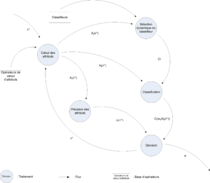
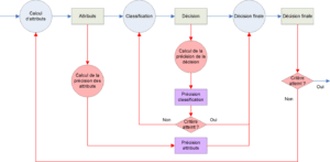
The belief functions per class/classifier/attribute are combined (Dempster) to construct a belief function per class. The decision is then made according to equation 3.3.3. The decision mechanism is illustrated in figure 4.2.1. This figure shows the sequence of processes and the exchanges between them. Each variable in the formalism is represented here, along with its origin and destination. The source of the flow illustrating the individual to be analyzed () is not shown, as we are not dealing with this part. can be an object injected directly into the process, but it can also be the result of subsequent processing.

The exploitation of Appriou’s expression, and our modified version of Appriou’s expression, exploits discrete labels based on the likelihood function linking an individual to its membership of the class .

In order to obtain these functions, and according to the diagram in figure 4.2.2, these labels are in our case derived from a classification stage linking the individual to the class. Classically in this framework, the likelihood function is then linked to the distance of the individual to the class according to the classifier (depending on the classifier, the distance can be replaced by a degree of membership or a probability). However, the ability to associate an individual with a label by a classifier is dependent on the attribute set used. Similarly, each classifier proposes a different partitioning of the attribute space, depending on the class model used or the metrics implemented. We will therefore relate the likelihood function to the distance , where represents the vector of attributes provided by the operator (Zernike moments of order 15, for example, or a 32-bin color histogram obtained by fuzzy C-means, etc.) and refers to the classifier.

The choice of this script allows us to combine several labels from different classifiers and/or different attributes. Depending on the chosen protocol, the different classifiers will either compete directly with each other, or a dynamic selection of the best classifier will take place before the merging step. In the latter case, the competition merges the labels from different attributes seen through the best classifier for each of them. The expression we arrive at is directly deduced from equation 3.3.3 :

(4.2.1)  

Appriou incorporates , a normalization parameter of the formula established so that the belief mass is between 0 and 1. is therefore a value between and the maximum value that can be estimated for . This value of is unique for classifier and corresponds to the greatest distance identified or possible between an individual and the classes defined for this classifier, hence:
\begin {eqnarray}
\nonumber\mbox{for }0\leq 1-\frac{x}{y}\leq 1\mbox{ it is necessary }y\geq x\
\nonumber\mbox{ hence }y=sup_x(\max_q(C_i(\omega_q|A_j(x))))\
0<R\leq\frac{1}{\sup_x(\max_q(C_i(\omega_q|A_j(x))))}
\tag{4.2.2}
\end{eqnarray}

The belief mass we’ve just established is , i.e. the belief mass associated with the fact that class is assigned to individual by classifier for attribute vector . What we’re interested in is the final decision to assign the class to the individual , and consequently the mass of belief in the class , , and the associated masses and :

(4.2.3)  

Based on Dempster’s combination model, we formalize this decision making from intermediate decisions on a set of labels for a single set of attributes:

(4.2.4)  

and :

(4.2.5)  

More generally, in the presence of several sets of attributes from different operators (or different parameters), Dempster’s combination rule leads to the general formulation :

(4.2.6)  

The data flow diagram in figure 4.2.1 illustrates how this script works.

Bibliography

[1] A. Appriou. Probabilities and uncertainties in multi-sensor data fusion. Revue Scientifique et Technique de la Défense, 11 :27-40, 1991.
[2] D. Arrivault. Apport des graphes dans la reconnaissance non-contrainte de caractères manuscrits anciens. PhD thesis, Université de Poitiers, 2002.
[3] I. Bloch. Fusion d’informations numériques: panorama méthodologique. In Journées Nationales de la Recherche en Robotique, 2005.[7]
[4] R. Caruana and A. Niculescu-Mizil. An empirical comparison of supervised learning algorithms. In ICML ’06: Proceedings of the 23rd international conference on Machine learning, pages 161-168, New York, NY, USA, 2006. ACM.
[5] T. M. Cover and P. E. Hart. Nearest neighbor pattern classification. IEEE Trans. on Information Theory 13(1):21-27, 1967.
[6] A. P. Dempster. Upper and lower probabilities induced by multiple valued mappings. Annals of Mathematical Statistics, 38 :325-339, 1967.
[7] A. P. Dempster. A generalization of bayesian inference. Journal of the Royal Statistical Society, 30 :205-247, 1968.
[8] T. Denœux. Analysis of evidence-theoretic decision rules for pattern classification. Pattern Recognition, 30(7) :1095-1107, 1997.
[9] J. Kholas and P. A. Monney. Lecture Notes in Economics and Mathematical Systems, volume 425, chapter A mathematical theory of hints: An approach to the Dempster-Shafer theory of evidence. Springer-Verlag, 1995.
[10] G. J. Klir and M. J. Wierman. Uncertainty-based information. Elements of generalized information theory, 2nd edition. Studies in fuzzyness and soft computing . Physica-Verlag, 1999.
[11] E. Lefevre, O. Colot, and P. Vannoorenberghe. Belief function combination and conflict management. Information Fusion, 3 :149-162, 2002.
[12] D. Mercier, B. Quost, and T. Denoœux. Refined modeling of sensor reliability in the belief function framework using contextual discounting. Information Fusion, 2007.
[13] E. Ramasso. Recognition of state sequences by the Transferable Belief Model – Application to the analysis of athletics videos. PhD thesis, Université Joseph Fourier de Grenoble, 2007.
[14] I. Rish. An empirical study of the naive bayes classifier. In IJCAI-01 workshop on “Empirical Methods in AI”, 2001.
[15] G. Shafer. A Mathematical Theory of Evidence. Princeton University Press, 1976.
[16] P. Smets. Beliefs functions: The disjunctive rule of combination and the generalized bayesian theorem. Int. Jour. of Approximate Reasoning 9 :1-35, 1993.
[17] P. Smets. The nature of the unnormalized beliefs encountered in the transferable belief model. In Proceedings of the 8th Annual Conference on Uncertainty in Artificial Intelligence, pages 292-297, 1992.
[18] P. Smets. Advances in the Dempster-Shafer Theory of Evidence – What is Dempster-Shafer’s model? Wiley, 1994.
[19] P. Smets. Decision making in the tbm: The necessity of the pignistic transformation. Int. Jour. of Approximate Reasoning 38 :133-147, 2005.
[20] P. Smets and R. Kennes. The transferable belief model. Artificial Intelligence, 66(2) :191-234, 1994.
[21] B. Yaghlane, P. Smets, and K. Mellouli. Yaghlane, P. Smets, and K. Mellouli. Belief function independence: I. the marginal case. Int. Jour. of Approximate Reasoning 29 :47-70, 2001.
[22] B. Yaghlane, P. Smets, and K. Mellouli. Belief function independence : II. the conditionnal case. Int. Jour. of Approximate Reasoning 31(1) :31-75, 2002.
[23] B. Yaghlane, P. Smets, and K. Mellouli. Independence concept for belief functions. In Physica-Verlag, editor, Technologies for constructing intelligent systems : Tools, 2002 [93].

Proposal for a Regulation of the European Parliament and of the Council laying down harmonized rules on artificial intelligence (artificial intelligence legislation) and amending certain Union legislative acts

ISO/IEC 42001